Loading OpenBCI datasets in EEGLAB

EEGLAB can be used for the analysis and visualization of EEG datasets recorded using OpenBCI hardware and software. EEGLAB can work with a variety of different file types, including those that are exported from the OpenBCI GUI, as we saw in the previous post.

The Approach

The main goal of this post is to explain how to upload OpenBCI datasets in EEGLAB in a simple, easy and straightforward way. Before that, we need to know some important facts related to data files and MATLAB data requirements:

• The OpenBCI GUI saves the raw data in an ASCII file, either with a “.txt’ or “.csv” extension.  You can select your preference in the “SavedData.pde” tab from the OpenBCI GUI files written in Processing (Java).
• EEGLAB (MATLAB Toolbox) requires that the channel information is saved in columns (not rows). Good news is that OpenBCI raw data files are saved exactly like this. So, we only need to select to significant data into the files and upload it in EEGLAB, and there is no need to transpose it. You can read more information about the EEGLAB data requirements here.

Taking into account the conditions and information wrote above, I wrote a MATLAB script that opens an OpenBCI data file, and it saves the EEG information in a MATLAB variable (“.mat”) or in a CSV file (“.csv”). You only need to run the script and you will be able to import directly the file to EEGLAB. Besides, you can also filter the EEG signal (low, high, and notch filters), and plot the EEG signal (both filtered and non-filtered). You can find and download it here.

MATLAB

Once you have downloaded the script, you will see different MATLAb files inside the folder. The main_program_8ch is the principal MATLAB script that calls the open_files and bandpass_filter_8ch functions. If you want to plot the EEG data you must run the plots_8ch script, but do not clean the variables from your workspace.

There is only one step that needs to be done in MATLAB, and it’s to run the main script:

> main_program_8ch

The first line in the main script relies on the open_files function. This function has a pretty legit objective which is to let you navigate through your computer and select the file of interest without having to type the name every time.

function [data] = open_files()
  % Prompt user for filename
   [fname, fdir] = uigetfile( ...
   { '*.txt*', 'Text Files (*.txt*)'; ...
     '*.xlsx', 'Excel Files (*.xlsx)'; ...
     '*.csv*', 'Text Files (*.csv)'}, ...
     'Pick a file');
  % Create fully-formed filename as a string
   filename = fullfile(fdir, fname);
  % Check that file exists
   assert(exist(filename, 'file') == 2, '%s does not exist.', filename);
  % Read in the data, skipping the 5 first rows
   data = csvread(filename,5,0);
end

The line data = csvread(filename,5,0) skips the first five rows of the OpenBCI text file. The row offset is the number of rows in your text file before the start of your EEG data (in the current version of the OpenBCI GUI, there are 5 commented lines before the start of the data, so the offset should be 5 to make the matrix start on line 6). Column offset skips the sample number column.

A window will pop-up on your screen. It will ask you to pick a file and it will give you three options, involving “.txt”, “.csv”, and “.xlsx” extensions formats. By default, OpenBCI saves its raw data in “.txt”, so you can select “.txt” option, navigate to the “Saved data” folder in the OpenBCI GUI folder, and select the file of interest.

Figure 2. A window will pop-up after running the main script and it will ask you to pick the file of interest. You have three possible extension formats.

Immediately, you will see that you have eleven new variables in your workspace, and two new MATLAB (“.mat”) variables saved in the current folder.

Figure 3. The result after running the MATLAB script.

Three things basically happened once we imported the OpenBCI file to MATLAB:

• New variables were created. The EEG data was selected from columns 2 to 9, and so it was done for the auxiliary data from columns 10 to 12 (this might be useful in case you have information of interest saved in them).

% Separate EEG data and auxiliary data 
  eegdata = data(:,2:9);            % EEG data
  auxdata = data(:,10:12);          % Aux data

Moreover, a time vector is created based on the “eegdata” variable length that will be used in the plots_8ch script (in case you want to visualize your EEG data in Matlab first). Also, information about the filters is created.

% General variables
 time = (0:4:length(eegdata))';      % Time vector
 N_ch = 8;                           % Number of channels

% Band-pass Filtering Paramaters
 fsamp = 250;                        % Sampling frequency
 tsample = 1/fsamp;                  % Period of samples
 f_low = 50;                         % Cut frequency for high-pass filter
 f_high = 1;                         % Cut frequency for low-pass filter

• The EEG data was filtered. In case you want to filter the data before importing the files to EEGLAB, I created this function where the raw data is filtered with a low-pass, a high-pass, and a notch filter. Feel free to change the cut-off frequencies for all the filters.

% Bandpass Filter
  for i=1:N_ch
    EEG(:,i)= bandpass_filter_8ch(eegdata(:,i), fsamp, f_low, f_high);
  end

First of all, a low-pass filtered is applied, followed by a high-pass filtered. Afterward, a Notch filter is applied to the data so as to eliminate the DC artifacts. The output variable with the EEG data filtered is called “EEG”.

function [EEG] = bandpass_filter_8ch(eeg_data, fsamp, f_low, f_high)
  N_ch=size(eeg_data,2);
  order = 2;

  % Low-pass EEG filter
    [b,a]=butter(2,2*f_low/fsamp,'low');
     for i=1:N_ch
      eeg_data(:,i)=transpose(filtfilt(b,a,eeg_data(:,i)));
     end

  % High-pass EEG filter
    [b1,a1]=butter(2,2*f_high/fsamp,'high');
     for i=1:N_ch
      eeg_data2(:,i)=transpose(filtfilt(b1,a1,eeg_data(:,i)));
     end

  % Notch filter
    Wn = [58 62]/fsamp*2; % Cutoff frequencies
    [bn,an] = butter(order,Wn,'stop'); % Calculate filter coefficients
     for i=1:N_ch
      EEG(:,i)=transpose(filtfilt(bn,an,eeg_data2(:,i)));
     end
end

• The EEG data was saved.

Both the filtered (“EEG”) and the non-filtered (“eegdata”) EEG data are saved as Matlab variables in the current folder. For example, the “eegdata.mat” variable should look like the figure below. You will notice that the channel information is saved in columns.

% Save raw data (unfiltered data)
save('eegdata.csv','eegdata');
save('eegdata.mat','eegdata');

% Save filterd data
save('EEG.csv','EEG');
save('EEG.mat','EEG');

Figure 4. Your EEG data should look like this. The channel information is saved in columns (not rows).

Now we are ready to import the data from the OpenBCI GUI in EEGLAB!

EEGLAB

If EEGLAB isn’t already running, type the following line into the Matlab command line to start the program, and check that you are in the correct path before you run it.

> eeglab

A little blue window will pop-up in your screen, such as the one tha appears below. To import the Matlab variable that you saved earlier, go to File -> Import Data -> Using EEGLAB functions and plugins -> From ASCII/float file or Matlab array.

Figure 5. Importing data to EEGLAB. From EEGLAB.

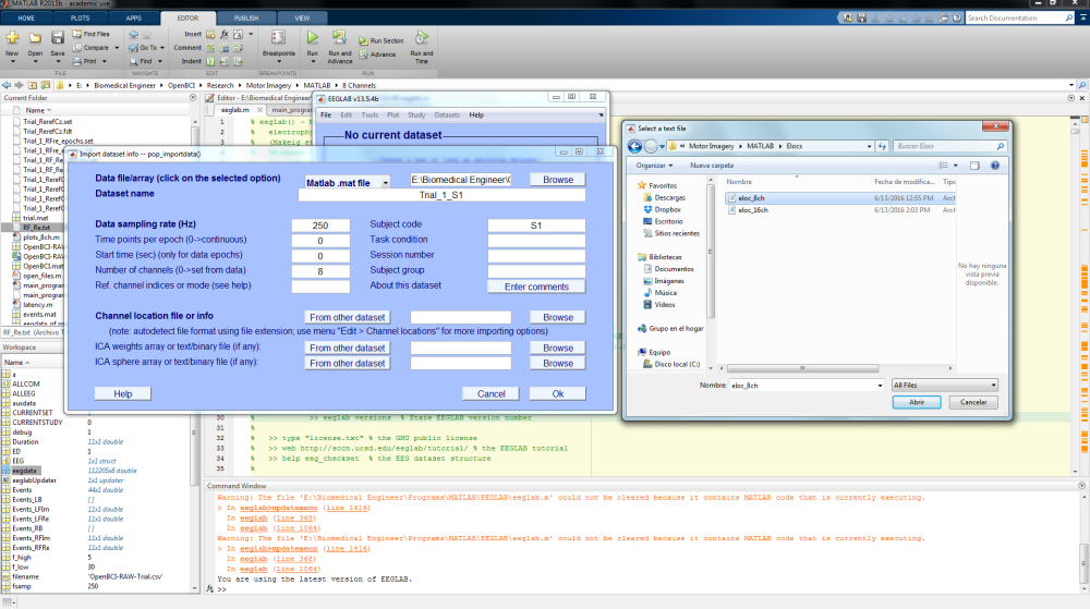
Another window will pop-up asking for information about the dataset that you want to create. Let’s first upload the EEG data variable. Select “Matlab variable”, and browse to the current folder where we saved the variables and select either “EEG.mat” or “eegdata.mat”. Don’t forget to type the Data Sampling rate (it should be commented in at the top of the “.txt” file – usually 250 Hz by default in the OpenBCI GUI). The other fields can be left at default, and EEGLAB will automatically fill in the information from the data set.

Figure 6. Select the EEG data and Channel Locations files.

Channel locations are useful for plotting EEG scalp maps in 2-D or 3-D format. OpenBCI uses the standard 10-20 format for the 8 and 16 channel models, which can be found within these .ced files: 8 channel and 16 channel. You can then import channel data by click “Browse” next to “Channel location file or info” and locating the OpenBCI .ced file you downloaded.

Figure 5. My 8 Channel locations file in .ced format.

If you need to edit the channel locations, I would suggest you editing either “eeglab_chan32.locs” located in “\EEGLAB\sample_data” or “Standard-10-20-Cap25.ced” located in “\EEGLAB\sample_locs”. You should use any text editors such as WordPad, NotePad++, Atom… Whichever works better for you and edit the files.

Congratulations! The data is now imported into EEGLAB, and you can perform a variety of data analysis on the data. See (Performing EEG data analysis and visualization) for next steps on working with your data.

References

• EEGLAB Import Data requirements – link
• Save CSV in MATLAB – link